40 how to arrange row labels in pivot table

Repeat item labels in a PivotTable - support.microsoft.com Right-click the row or column label you want to repeat, and click Field Settings. Click the Layout & Print tab, and check the Repeat item labels box. Make sure Show item labels in tabular form is selected. Notes: When you edit any of the repeated labels, the changes you make are applied to all other cells with the same label. How to Sort Pivot Table Columns and Rows - EDUCBA To sort any pivot table, there are 2 ways. First, we can click right the pivot table field we want to sort and select the appropriate option from the Sort by list. Also, we can choose More Sort Options from the same list to sort more. Another way is by applying the filter in a Pivot table.

Excel Pivot Tables - Sorting Data - tutorialspoint.com You can sort the data in the above PivotTable on Fields that are in Rows or Columns - Region, Salesperson and Month. To sort the PivotTable with the field Salesperson, proceed as follows −. Click the arrow in the Row Labels. Select Salesperson in the Select Field box from the dropdown list. More Sort Options.

How to arrange row labels in pivot table

How to Use Excel Pivot Table Label Filters To change the Pivot Table option, and allow multiple filters, follow these steps: Right-click a cell in the pivot table, and click PivotTable Options. In the PivotTable Options dialog box, click the Totals & Filters tab. In the Filters section, add a check mark to 'Allow multiple filters per field.'. Click the OK button, to apply the setting ... multiple fields as row labels on the same level in pivot table Excel ... I created a table below similar to how my data is (except with way more columns in my actual sheet). What I want to do is list all of Part A #s with the monthly volume for each, below that Part B #s with monthly volume, and below that Part C #s with monthly volume and so on, with Part A through Part E listed under the same column in the pivot. Filtering row labels in pivot table using vba - Stack Overflow In order to find the appropriate name, please run the following code: For each pField in ActiveSheet.PivotTables ("PivotTable1").PivotFields Debug.Print pField.Name Next pField. Go to VBA Editor, press Ctrl+G, it will open the immediate window. It will show all the available pivot fields.Then please use the correct Pivot Field and try. Share ...

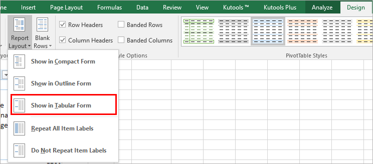
How to arrange row labels in pivot table. Pivot table row labels in separate columns • AuditExcel.co.za So when you click in the Pivot Table and click on the DESIGN tab one of the options is the Report Layout. Click on this and change it to Tabular form. Your pivot table report will now look like the bottom picture and will be easier to use in other areas of the spreadsheet and in our opinion is also easier to read. How to Customize Your Excel Pivot Chart Data Labels - dummies To remove the labels, select the None command. If you want to specify what Excel should use for the data label, choose the More Data Labels Options command from the Data Labels menu. Excel displays the Format Data Labels pane. Check the box that corresponds to the bit of pivot table or Excel table information that you want to use as the label. Sort an Excel Pivot Table Manually | MyExcelOnline DOWNLOAD EXCEL WORKBOOK. STEP 1: To manually sort a row, click on the cell you want to move. Hover over the border of that cell until you see the four arrows: Left mouse click, hold and drag it to the position you want (i.e. upwards to the first row) We dragged it to the top so it's now the first row! STEP 2: To manually sort a column, click ... How to Add Rows to a Pivot Table: 9 Steps (with Pictures) Click anywhere in your pivot table. This opens the pivot table editor on the right side of Google Sheets. 3. Click Add under "Rows." It's in the left side of the pivot table editor. A list of fields will expand on the menu. 4. Click the name of the field you want to add as a row.

Manually Sorting Pivot Table Row Labels In the Sort dialog box, select the type of sort that you want by doing one of the following: To return items to their original order, click Data source order. This option is only available for OLAP source data. To drag and arrange items the way that you want, click Manual. Excel: How to Sort Pivot Table by Date - Statology The rows in the pivot table will automatically be sorted from newest to oldest: To sort from oldest date to newest date, simply click the dropdown arrow next to Row Labels again and then click Sort Oldest to Newest. Additional Resources. The following tutorials explain how to perform other common operations in Excel: Excel tutorial: How to filter a pivot table by rows or columns Let's take a look. This pivot table is displaying just one field: Total Sales. After we add Product as a row label, notice that a drop-down arrow appears in the header area. When we open this menu, we see a variety of filter options. The simplest way to filter is to simply include or exclude items by using the checklist that appears below. How to add side by side rows in excel pivot table - AnswerTabs To display more pivot table rows side by side, you need to turn on the Classic PivotTable layout and modify Field settings. For example will be used the following table: You have to right-click on pivot table and choose the PivotTable options. Then swich to Display tab and turn on Classic PivotTable layout:

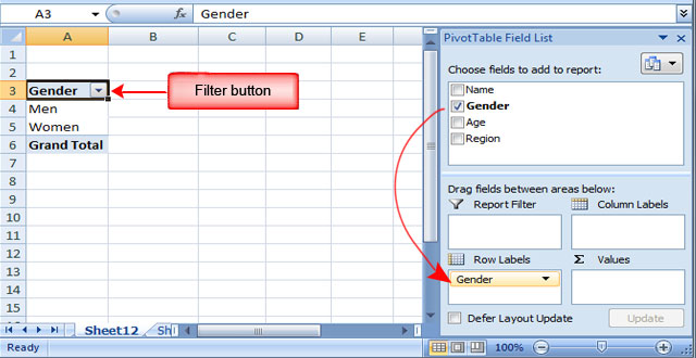
How to rename group or row labels in Excel PivotTable? 1. Click at the PivotTable, then click Analyze tab and go to the Active Field textbox. 2. Now in the Active Field textbox, the active field name is displayed, you can change it in the textbox. You can change other Row Labels name by clicking the relative fields in the PivotTable, then rename it in the Active Field textbox. How to create row labels for a PivotTable? - Stack Overflow I need to create a PivotTable such that in the Row labels are name and state, to look like this: name state income Steeve IL 3000 Mary CA 10000 Alex DC 11000 Michael Al 2000 ............. Automatic Row And Column Pivot Table Labels - How To Excel At Excel Select the data set you want to use for your table; The first thing to do is put your cursor somewhere in your data list; Select the Insert Tab; Hit Pivot Table icon; Next select Pivot Table option; Select a table or range option; Select to put your Table on a New Worksheet or on the current one, for this tutorial select the first option; Click Ok Grouping, sorting, and filtering pivot data - Microsoft Press Store The pivot table in that figure is using Tabular layout. If your pivot tables use Compact layout, you see a drop-down menu on the cell with Row Labels or Column Labels. If you have multiple row fields, it is just as easy to sort using the invisible drop-down menus that appear when you hover over a field in the top of the PivotTable Fields list.

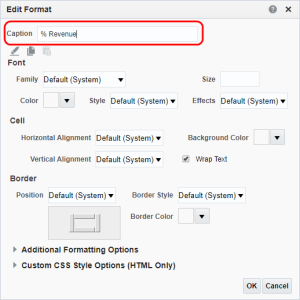
Formatting a pivot table and adding calculations

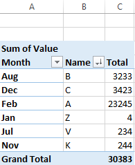
Sorting Row Labels in a Pivot Table by Month - Microsoft Community Sorting Row Labels in a Pivot Table by Month Hoping somebody can help please. I have a Dataset with dates people book holidays. I have a column using the =TEXT (A1,"mmm-yy") to get them grouped by month. I thine put that column in a pivot table but the table doesn't go from January -December. It does it by the first letter so April, Aug, Feb etc.,

Arrange Pivot Table Data Vertically - Excel Pivot TablesExcel Pivot Tables

Move Row Labels in Pivot Table - Excel Pivot Tables When you add fields to the row labels area in a pivot table, the field's items are automatically sorted. See how you can manually move those labels, to put them in a different order. There's a video and written steps below. In the screen shot below, the districts are listed alphabetically, from Central to West. Change the Order

Sort multiple row label in pivot table - Microsoft Community

How to Move Excel Pivot Table Labels Quick Tricks Click on the cell where you want a different label to appear Type the name of the label that you want to move Press Enter The existing labels shift down, and the moved label takes its new position. For example, type "West" in cell A4, over the existing District name, "Central" Then, press Enter, to complete the change.

Pivot Table Multiple Row Labels Side By Side | Decorations I Can Make

Design the layout and format of a PivotTable On the Options tab, in the PivotTable group, click Options. In the PivotTable Options dialog box, click the Layout & Format tab, and then under Layout, select or clear the Merge and center cells with labels check box. Note: You cannot use the Merge Cells check box under the Alignment tab in a PivotTable.

How to Sort Pivot Table Row Labels, Column Field Labels and Data Values with Excel VBA Macro ...

Pivot Table Row Labels In the Same Line - Beat Excel! First make a pivot table with required fields. Arrange the fields as shown in left picture. Your initial table will look like right picture. Now click on "Error Code" and access field settings. First check "None" option in "Subtotals & Filters" tab to disable totals after every row.

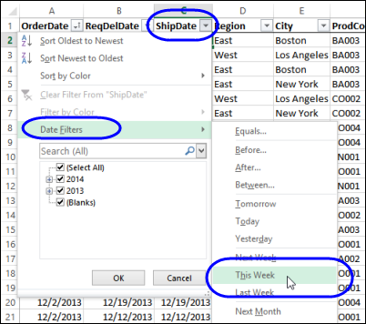
Dynamic Date Range Filters in Pivot Table - Excel Pivot TablesExcel Pivot Tables

Excel tutorial: How to rearrange fields in a pivot table In this pivot table, we have the Product field in the Row Labels area and Region in the Column Labels areas. We can just drag the fields to swap locations. And drag them back again to restore the original orientation. In this same way, we can look at product sales by region and state by adding State to the Column labels area.

Repeat Pivot Table row labels • AuditExcel.co.za Pivot Tables Course

Pivot table row labels side by side - Excel Tutorials Now, let's create a pivot table ( Insert >> Tables >> Pivot Table) and check all the values in Pivot Table Fields. Fields should look like this. Right-click inside a pivot table and choose PivotTable Options…. Check data as shown on the image below. The table is going to change. The pivot table is almost ready.

Excel 2010 - Pivot Table - How to print repeating row labels at the top of every new page

How to make row labels on same line in pivot table? 1. Click any one cell in the pivot table, and right click to choose PivotTable Options, see screenshot: 2. In the PivotTable Options dialog box, click the Display tab, and then check Classic PivotTable layout (enables... 3. Then click OK to close this dialog, and you will get the following pivot ...

How To Create A Pivot Table With Multiple Columns And Rows | Awesome Home

Sorting to your Pivot table row labels in custom order [quick tip] Using MATCH formula, find the order of each row label (in our case, classification) in the sort order list. Assuming classification is in D3, use =MATCH (D3, $I$3:$I$12, 0) Create a pivot table with data set including sort order column. Add sort order column along with classification to the pivot table row labels area.

Pivot Tables Excel 2007 Row Labels Side By | Brokeasshome.com

Filtering row labels in pivot table using vba - Stack Overflow In order to find the appropriate name, please run the following code: For each pField in ActiveSheet.PivotTables ("PivotTable1").PivotFields Debug.Print pField.Name Next pField. Go to VBA Editor, press Ctrl+G, it will open the immediate window. It will show all the available pivot fields.Then please use the correct Pivot Field and try. Share ...

Excel Pivot Table Report - Sort Data in Row & Column Labels & in Values Area, use Custom Lists

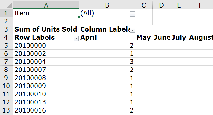
multiple fields as row labels on the same level in pivot table Excel ... I created a table below similar to how my data is (except with way more columns in my actual sheet). What I want to do is list all of Part A #s with the monthly volume for each, below that Part B #s with monthly volume, and below that Part C #s with monthly volume and so on, with Part A through Part E listed under the same column in the pivot.