45 update data labels in excel chart

Creating a chart with dynamic labels - Microsoft Excel 2016 1. Right-click on the chart and in the popup menu, select Add Data Labels and again Add Data Labels : 2. Do one of the following: For all labels: on the Format Data Labels pane, in the Label Options, in the Label Contains group, check Value From Cells and then choose cells: For the specific label: double-click on the label value, in the popup ... How to add or move data labels in Excel chart? - ExtendOffice In Excel 2013 or 2016. 1. Click the chart to show the Chart Elements button . 2. Then click the Chart Elements, and check Data Labels, then you can click the arrow to choose an option about the data labels in the sub menu. See screenshot: In Excel 2010 or 2007. 1. click on the chart to show the Layout tab in the Chart Tools group. See ...

› charts › variance-clusteredActual vs Budget or Target Chart in Excel - Variance on ... Aug 19, 2013 · Set Data Labels to Cell Values Screenshot Excel 2003-2010. The nice part about either of these methods is that the data labels are linked to the values in the cells. If your numbers change or you update the data, the labels will automatically be refreshed and display the correct results. Please let me know if you have any questions.

Update data labels in excel chart

how to add data label automatically | Chandoo.org Excel Forums - Become ... hi all, i have a question regarding data label, lets just say we have something to be input as line chart in every week and we want to show the latest week value in the line chart, normally what i do is i select the latest dot in line chart and click add data label, then delete the previous... trumpexcel.com › dynamic-chart-rangeHow to Create a Dynamic Chart Range in Excel Here are the exact steps to create a dynamic line chart using the Excel table: Select the entire Excel table. Go to the Insert tab. In the Charts Group, select ‘Line with Markers’ chart. That’s it! The above steps would insert a line chart which would automatically update when you add more data to the Excel table. Excel Chart - Selecting and updating ALL data labels - Right-click a "point" in the series, which actually will be a bar piece - Choose add data labels - Right-click again and choose format data labels - Check series name - Uncheck value That's it…. You must log in or register to reply here. Excel contains over 450 functions, with more added every year.

Update data labels in excel chart. Excel Charts: Creating Custom Data Labels - YouTube In this video I'll show you how to add data labels to a chart in Excel and then change the range that the data labels are linked to. This video covers both W... How to auto update a chart after entering new data in Excel? Auto update a chart after entering new data with creating a table If you have the following range of data and column chart, now you want the chart update automatically when you enter new information. In Excel 2007, 2010 or 2013, you can create a table to expand the data range, and the chart will update automatically. Please do as this: 1. How to Customize Your Excel Pivot Chart Data Labels - dummies The Data Labels command on the Design tab's Add Chart Element menu in Excel allows you to label data markers with values from your pivot table. When you click the command button, Excel displays a menu with commands corresponding to locations for the data labels: None, Center, Left, Right, Above, and Below. None signifies that no data labels ... How to add data labels from different column in an Excel chart? Right click the data series in the chart, and select Add Data Labels > Add Data Labels from the context menu to add data labels. 2. Click any data label to select all data labels, and then click the specified data label to select it only in the chart. 3.

Change the format of data labels in a chart To get there, after adding your data labels, select the data label to format, and then click Chart Elements > Data Labels > More Options. To go to the appropriate area, click one of the four icons ( Fill & Line, Effects, Size & Properties ( Layout & Properties in Outlook or Word), or Label Options) shown here. chandoo.org › wp › change-data-labels-in-chartsHow to Change Excel Chart Data Labels to Custom Values? May 05, 2010 · Now, click on any data label. This will select “all” data labels. Now click once again. At this point excel will select only one data label. Go to Formula bar, press = and point to the cell where the data label for that chart data point is defined. Repeat the process for all other data labels, one after another. See the screencast. excel - How do I update the data label of a chart? - Stack Overflow Select the data label Then, place your cursor in Excel's Formula Bar, and enter the formula like ='Sheet2'!$C$3. Now, that data label is associated by the formula, to the cell C3, which contains the desired data label that we built above. Repeat as needed. Note: The sheet name is required in this formula. Missing Charts Data Labels After Office 365 Proplus Update Missing data labels on an Excel chart linked to a PowerPoint presentation could be due to the recent update changing some settings in the app or data got corrupted. As an initial recommendation to assist in resolving your concern, kindly follow the steps below to reset the data label text being shown: Click on the chart.

Excel Chart: Horizontal Axis Labels won't update I created the data set in Excel 2016, selected the data and inserted a line chart. I sent one line to the secondary axis. The X axis still shows the correct labels. I sent the other line to the secondary axis and brought the first line back to the primary axis. The X axis labels are still correct. In short, I cannot reproduce the problem. support.microsoft.com › en-us › officeInsert a chart from an Excel spreadsheet into Word To update the chart automatically, change the data in the embedded workbook. Keep Source Formatting & Embed Workbook. Keeps the Excel theme. Embeds a copy of the Excel workbook with the chart. The chart doesn’t stay linked to the original workbook. To update the chart automatically, change the data in the embedded workbook. Add or remove data labels in a chart - support.microsoft.com Click the data series or chart. To label one data point, after clicking the series, click that data point. In the upper right corner, next to the chart, click Add Chart Element > Data Labels. To change the location, click the arrow, and choose an option. If you want to show your data label inside a text bubble shape, click Data Callout. Adding Data Labels to a Chart Using VBA Loops - Wise Owl One way to do this is by manually adding data labels to the chart within Excel, but we're going to achieve the same result in a single line of code. To do this, add the following line to your code: 'make sure data labels are turned on FilmDataSeries.HasDataLabels = True

How to Add a Third Y-Axis to a Scatter Chart | EngineerExcel

Data Labels - Value From Cells - Text Not Updating Sign in to vote The data labels in the excel are not updating after changing the data scenario: It is always we need to format data labels, reset label text, uncheck and recheck the value from cells box. So whether latest version of 2019 has updated this bug or is it still pending to be addressed?

Excel - Line Chart

Automatically update data labels on Excel chart (Excel 2016) Impact x axis, probability y axis, and ref as the data label. I formated data labels using "values from cell" command on the REF column (highlighting all the data, including the blank cells). All the data in this table are lookups from other tables if that matters.

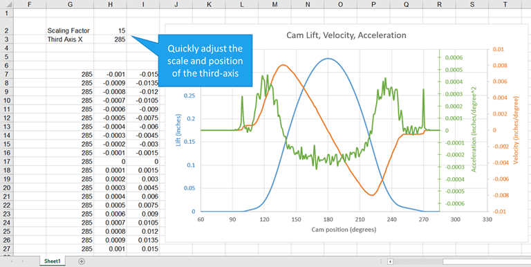
How to Add a Third Y-Axis to a Scatter Chart | EngineerExcel

How to Use Cell Values for Excel Chart Labels Select the chart, choose the "Chart Elements" option, click the "Data Labels" arrow, and then "More Options." Uncheck the "Value" box and check the "Value From Cells" box. Select cells C2:C6 to use for the data label range and then click the "OK" button. The values from these cells are now used for the chart data labels.

Create a pie chart from distinct values in one column by grouping data in Excel - Super User

Edit titles or data labels in a chart - support.microsoft.com The first click selects the data labels for the whole data series, and the second click selects the individual data label. Right-click the data label, and then click Format Data Label or Format Data Labels. Click Label Options if it's not selected, and then select the Reset Label Text check box. Top of Page

Sunburst Chart in Excel

excelmate.wordpress.com › 2014/07/15 › 637Excel – Create a Dynamic 12 Month Rolling Chart | Excelmate Jul 15, 2014 · To create a dynamic chart using this simple table we will need two named dynamic ranges – one for the data itself and one for the labels. Note that when working with charts you will need to create a separate dynamic range for each series as charts treat each series separately so you cannot create a single dynamic named range that includes all rows and columns.

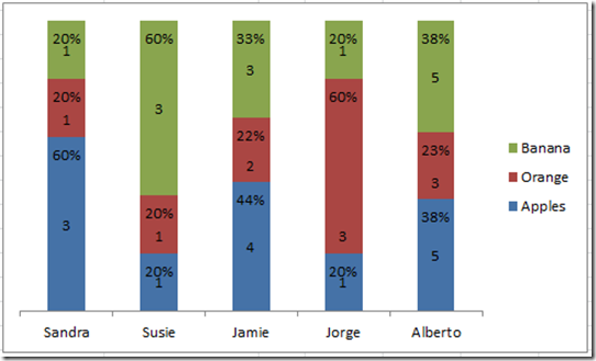
Friday Challenge - Create a Percentage (%) and Value Label within 100% Stacked Chart? - Excel ...

› ExcelTemplates › waterfall-chartWaterfall Chart Template for Excel - Vertex42.com Jul 02, 2015 · If the data labels don't end up where you want them, you can manually change the location of each individual data label by dragging them with your mouse. Formatting Data Labels The data labels for the negative adjustments use a custom number format of "-#,##0;-#,##0" to force the values to show the negative sign "-" even though the actual ...

Custom Data Labels with Colors and Symbols in Excel Charts - [How To] - PakAccountants.com

Update the data in an existing chart Changes you make will instantly show up in the chart. Right-click the item you want to change and input the data--or type a new heading--and press Enter to display it in the chart. To hide a category in the chart, right-click the chart and choose Select Data. Deselect the item in the list and select OK.

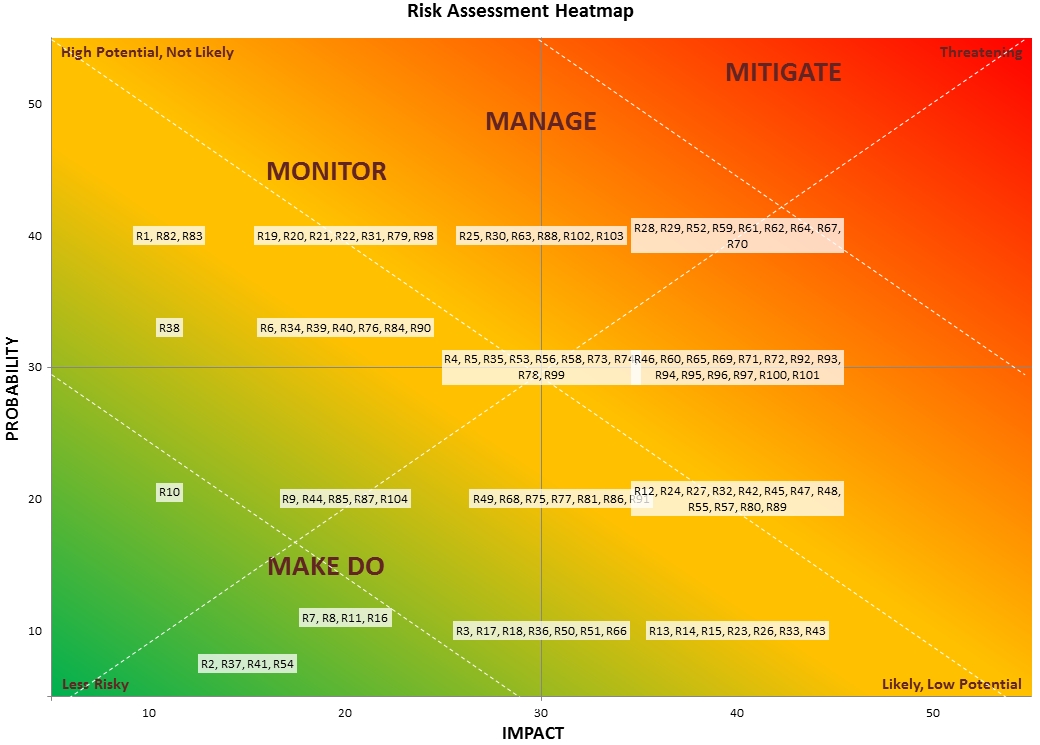
How to Create a Risk Heatmap in Excel - Part 2 - Risk Management Guru

How to add and customize chart data labels - Get Digital Help Edit data labels. Excel allows you to edit the data label value manually, simply press with left mouse button on a data label until it is selected. Press with left mouse button on again to select the text, you can now type any value you want. I changed the data label value to "Look here!". You can link a group of data labels to a cell range so ...

Share :